Implementing Windkessel Pressure Boundary Conditions in ANSYS Fluent Using UDFs
The pressure boundary conditions provided in the ANSYS Fluent graphical user interface (GUI) primarily support constant values or predefined transient waveforms [1]. However, in many applications, the outlet pressure evolves dynamically in response to the instantaneous flowrate through the cross-section. In this work, we impose a pressure boundary condition whose value varies according to the following equation:
\[\frac{dP(t)}{dt} = \frac{R_c+R_p}{R_p C}Q(t) + R_c\frac{dQ(t)}{dt}\]From the above equation, it can be seen that the pressure increment at the next time step depends on both the instantaneous flowrate and its temporal derivative, while the Windkessel parameters $R_c$, $R_p$, and $C$ are assumed to be known constants. The flowrate at the current time step can be obtained by integrating the flux over all faces on the outlet cross-section. However, evaluating the flowrate derivative requires the flowrate from the previous time step, which must therefore be stored in User-Defined Memory (UDM). The derivative can then be approximated using the following finite-difference expression:
\[\frac{dQ(t)}{dt} = \frac{Q(t)-Q(t-\Delta t)}{\Delta t}\]ANSYS Fluent provides a large number of User-Defined Function (UDF) macros for customizing solver behavior. Readers interested in additional macros and their functionalities are referred to the Fluent UDF Manual [2].
Macros whose names begin with DEFINE_XXXX are special macros that expand into function definitions during preprocessing. Therefore, they cannot be nested within other DEFINE_XXXX macros [3] (i.e., placing one DEFINE macro inside another DEFINE macro). In contrast, most non-DEFINE macros provided in the manual can be invoked anywhere within a UDF.
In the present implementation, only two DEFINE macros are required:
DEFINE_PROFILEDEFINE_EXECUTE_AT_ENDDEFINE_PROFILE is used to prescribe boundary-condition profiles, such as velocity or pressure boundary conditions.
Its syntax is
DEFINE_PROFILE(macroName, thread, index)
where:
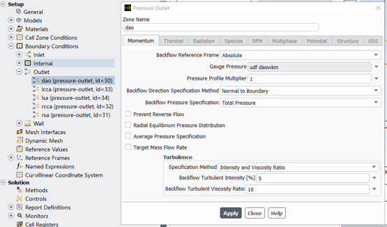
macroName: the name of the UDF. After the UDF is interpreted or compiled in Fluent, this name will appear in the corresponding boundary-condition dialog box, as illustrated in the figure below.thread: a pointer to the boundary zone (thread) to which the profile is applied.index: an integer index specifying which variable of the boundary condition is being modified.In Fluent, a thread represents a mesh zone, such as an inlet, outlet, wall, or fluid region. Understanding the concept of threads is essential for writing UDFs because most boundary operations are performed through them.
After the UDF is successfully loaded, the name specified by macroName becomes available in the Fluent GUI and can be assigned to the desired boundary condition, like the following screenshot:
thread is provided by ANSYS Fluent. For example, when a DEFINE_PROFILE UDF is hooked to a boundary condition through the graphical user interface (GUI), Fluent automatically passes a pointer to the corresponding boundary zone (thread) [4]. This thread contains all mesh entities associated with that zone, such as faces and their related information. The user can then access and process these data within the UDF.
index identifies the variable to be defined. The value of index is determined when the UDF is hooked to a variable in the boundary-condition dialog box. ANSYS Fluent subsequently passes this index to the UDF so that the function knows which variable (e.g., velocity, pressure, temperature, etc.) it should operate on.
For example:
DEFINE_PROFILE(boundary1, thread, index)
{
    face_t f;    // face_t is a Fluent data type representing a single face.

    begin_f_loop(f, thread)    // Loop over all faces in the specified thread.
    {
        F_PROFILE(f, thread, index) = 1.0;
        // Assign a value of 1.0 to the selected boundary variable on this face.
        // F_PROFILE is typically used together with DEFINE_PROFILE.
    }
    end_f_loop(f, thread);    // End of face loop.
}
In this example, the UDF loops over every face in the boundary zone represented by thread and assigns a constant value of 1.0 to the corresponding boundary variable identified by index.
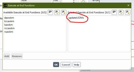
The other DEFINE macro used in this case is DEFINE_EXECUTE_AT_END(), which is executed at the end of each iteration for steady simulations or at the end of each time step for transient simulations.
Unlike DEFINE_PROFILE, this macro does not take any input arguments and is not automatically provided with any domain or thread information. Therefore, the user must explicitly obtain the required domain and thread pointers within the UDF.
In this work, we use the pressure-based coupled solver for transient flow simulations. The following figure illustrates the execution flow of ANSYS Fluent together with the UDFs used to achieve the Windkessel coupling:
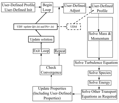
We do not use the User-Defined Adjust or User-Defined Properties hooks in this implementation, and therefore these steps can be ignored in the flowchart above.
During the User-Defined Profile stage, a DEFINE_PROFILE macro is assigned to each outlet boundary condition. At the end of each time step, the DEFINE_EXECUTE_AT_END macro is invoked to update the outlet pressure for the next time step, $P(t+\Delta t)$, and store the updated values in User-Defined Memory (UDM) [7].
As an example, consider a case with five outlets. Since one UDM is required to store the pressure history for each outlet, five UDM locations are needed for pressure storage.
Although Fluent provides macros for accessing cell-based quantities such as velocity and density from previous time steps, we did not find an equivalent macro for face-based quantities. Therefore, the flowrate on each face must be explicitly stored in UDM at the current time step and reused as the previous flowrate during the next time step.
Consequently, a total of ten UDM locations are required in this implementation: five for storing outlet pressures and five for storing face-based flow-rate information. The following table summarizes the purpose of each UDM location.
| UDM Location | Definition |
|---|---|
| 0 | RSA $Q(t-\Delta t)$ |
| 1 | RCCA $Q(t-\Delta t)$ |
| 2 | DAo $Q(t-\Delta t)$ |
| 3 | LCCA $Q(t-\Delta t)$ |
| 4 | LSA $Q(t-\Delta t)$ |
| 5 | RSA $P(t+\Delta t)$ |
| 6 | RCCA $P(t+\Delta t)$ |
| 7 | DAo $P(t+\Delta t)$ |
| 8 | LCCA $P(t+\Delta t)$ |
| 9 | LSA $P(t+\Delta t)$ |
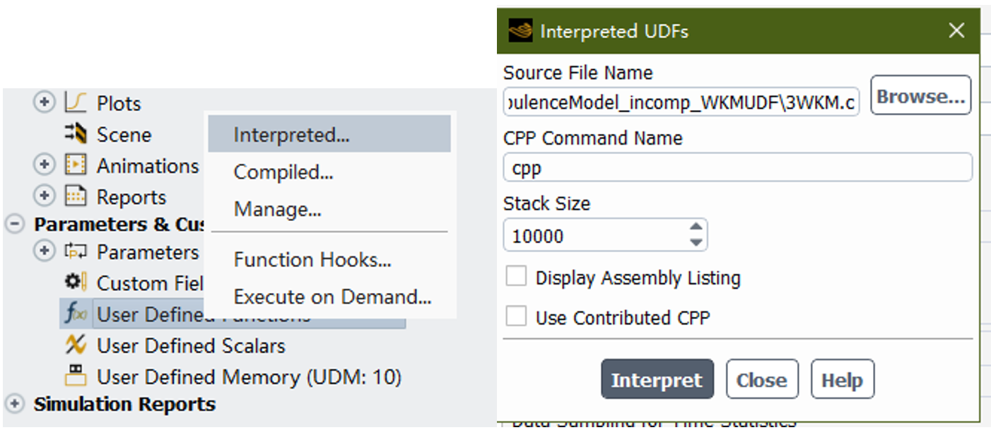
After the UDF has been implemented (the complete source code is provided in [8]), it can be imported into ANSYS Fluent. UDFs can be loaded using either the interpreted or compiled approach. Readers interested in the differences between these two methods are referred to the Fluent UDF Manual.
When using the compiled approach, it is recommended to replace printf() with Message(), especially for parallel simulations, as Message() provides more reliable output behavior in Fluent.
The following figures illustrate how to load and hook the UDF into the simulation.
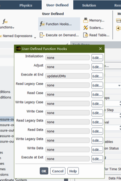
After the UDF has been successfully hooked, the Windkessel model is fully coupled with the transient CFD simulation.
The source code is provided in [8]. To adapt it to your own case, users may need to modify the following parameters:
R1ClinicalR2ClinicalCClinicalic, cm, mg, etc.)In addition, the thread IDs associated with the outlet boundaries must be updated to match those in your Fluent case. If your model contains a different number of outlets, corresponding modifications to the DEFINE_PROFILE macros and UDM assignments are also required.
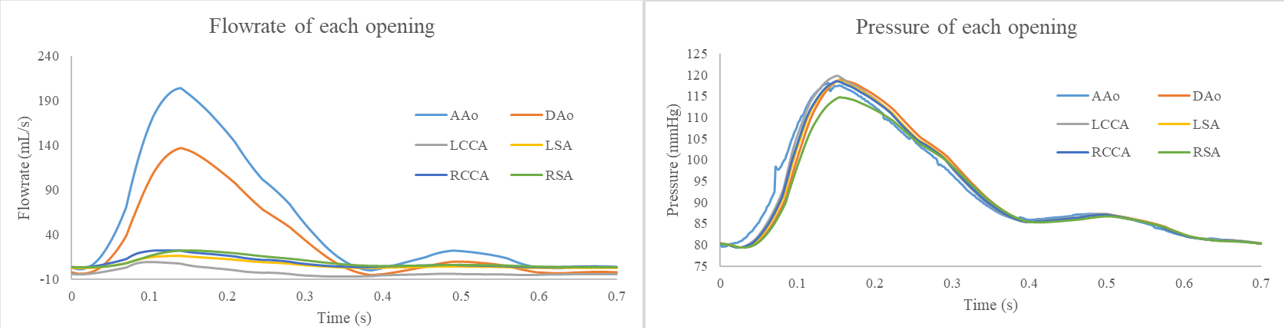
Finally, we examine the simulation results. By coupling the Windkessel model with the CFD solver, physiologically realistic flow distributions among the outlets are successfully achieved. The predicted pressure waveform at the ascending aorta (AAo) generally agrees with physiological expectations. However, the AAo pressure waveform exhibits small numerical artifacts during the systolic upstroke. These features are likely related to limited temporal or spatial resolution, although further investigation is required to identify their exact cause.
To prescribe a time-dependent waveform in ANSYS Fluent, a transient table can be imported from a text file. The file should follow the format below:
"table_name" "number_of_columns" "number_of_rows" "periodic_flag"
"column_1_name" "column_2_name"
"value_11" "value_12"
"value_21" "value_22"
"value_31" "value_32"
...
where:
table_name: the name that will appear in the Fluent GUI after the table is imported.number_of_columns: the total number of columns in the table.number_of_rows: the total number of data rows.periodic_flag: specifies whether the waveform is periodic (1) or non-periodic (0).For example:
vel 2 11 1
time vel
0 0
1 0.1
2 0.2
3 0.3
4 0.4
5 0.5
6 0.4
7 0.3
8 0.2
9 0.1
10 0
After creating the text file (e.g., velocity.txt), there are two ways to import it into Fluent.
The traditional approach is to place the file in
{project_directory}/dp0/FLTG/Fluent/
Alternatively, Fluent can also read a file using its full path.
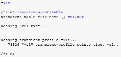
To import the transient table, open the Fluent console and enter:
/file/read-transient-table velocity.txt
or
/file/read-transient-table "C:/path/to/velocity.txt"
Once imported, the table becomes available for use in boundary-condition settings.
http://www.pmt.usp.br/academic/martoran/notasmodelosgrad/ANSYS%20Fluent%20UDF%20Manual.pdf
DEFINE_XXXX MacrosMultiple DEFINE_XXXX macros may coexist in a single source file. However, they cannot be nested within one another.
The following code is correct:
DEFINE_EXECUTE_AT_END(updateParameters)
{
    // Operations to be performed at the end of each time step.
}

DEFINE_PROFILE(boundary1, t, i)
{
    // Boundary-condition operations.
}
The following code is incorrect because one DEFINE macro is nested inside another:
DEFINE_EXECUTE_AT_END(updateParameters)
{
    DEFINE_PROFILE(boundary1, t, i)
    {
        // This is invalid.
    }
}
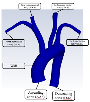
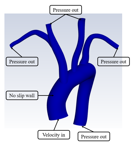
Consider the aortic flow case shown in the figure below. The computational domain consists of several boundary conditions, including a velocity inlet, pressure outlets, and no-slip walls. Together, these boundaries enclose the fluid domain.
Once the case and mesh are generated, Fluent organizes the computational mesh into several hierarchical data structures, including domain, thread, cell, face, node, and edge, as illustrated below.
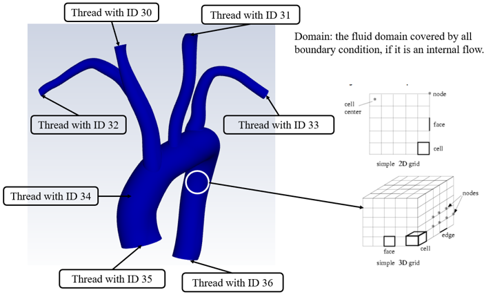
A domain typically represents the entire computational region. In a single-phase simulation, the fluid domain usually has an ID of 1, although this may vary depending on the simulation setup. The domain pointer can be obtained using the Get_Domain() macro [5].
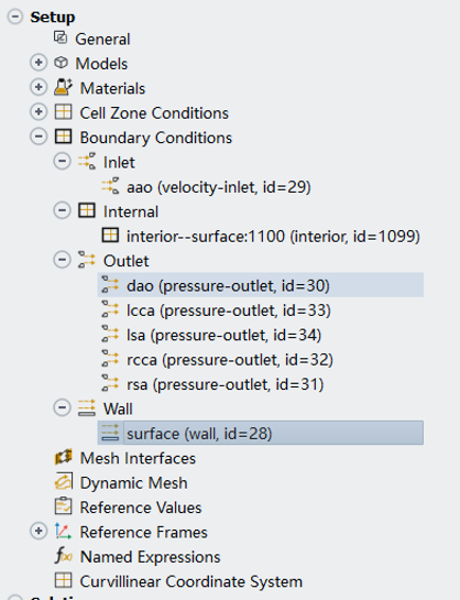
A thread represents a mesh zone in Fluent. A thread may correspond to a boundary zone (e.g., inlet, outlet, or wall) or a cell zone (e.g., fluid or solid region). Each thread is automatically assigned an integer ID by Fluent.
These thread IDs can be found in the Fluent GUI, as shown in the figure below.
Given a thread ID, the corresponding thread pointer can be obtained using the Lookup_Thread() macro [6]. Once the thread pointer is available, operations can be performed on the associated cells or faces.
In CFD simulations, most UDF operations are performed on cells and faces. In my experience and according to the Fluent UDF Manual, macros involving edges are relatively uncommon compared with those for cells and faces.
Some UDF macros, such as DEFINE_PROFILE, automatically receive domain or thread information as input arguments. However, other macros, such as DEFINE_EXECUTE_AT_END, do not provide any domain or thread pointers. In such cases, the user must explicitly obtain the desired domain.
The fluid domain can be obtained using the Get_Domain() macro:
Domain *d = Get_Domain(1);
The returned variable is a pointer to the domain. In many single-phase simulations, the fluid domain ID is typically 1, although this may vary depending on the case setup.
After obtaining the domain pointer, a specific thread can be retrieved if its thread ID is known. This is accomplished using the Lookup_Thread() macro:
Thread *t = Lookup_Thread(d, 30);
where:
d is the domain pointer.30 is the thread ID (for example, the outlet boundary with ID 30).The returned variable is a pointer to the corresponding thread. Once the thread pointer is available, operations can be performed on the associated cells or faces.
A typical workflow is therefore:
Domain *d = Get_Domain(1);
Thread *t = Lookup_Thread(d, 30);
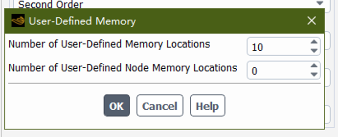
If UDMs are used in a UDF but have not been allocated before running the simulation, Fluent will report an error and may terminate the calculation.
To allocate UDM locations, navigate to:
User-Defined → Memory
and specify the number of UDM locations required by the UDF.
Fluent provides several macros for accessing UDM values. Common examples include:
F_UDMI(f, t, i) for face-based UDM access;C_UDMI(c, t, i) for cell-based UDM access.where:
f is a face of type face_t;c is a cell of type cell_t;t is the thread pointer;i is the UDM index.For example, suppose we want to assign a value of 1.0 to UDM location 0 for all faces belonging to thread 10:
Domain *d = Get_Domain(1);          // Obtain the fluid domain.
Thread *t = Lookup_Thread(d, 10);   // Obtain thread with ID 10.

face_t f;

begin_f_loop(f, t)
{
    F_UDMI(f, t, 0) = 1.0;          // Assign 1.0 to UDM location 0.
}
end_f_loop(f, t)
Similarly, for cell-based operations, replace:
begin_f_loop(f, t)
with
begin_c_loop(c, t)
and replace face_t with cell_t as appropriate.
The following UDF implements the Windkessel pressure boundary condition for five outlets. This implementation requires 10 UDM locations:
0–4: previous outlet flow rate, $Q_{\mathrm{prev}}$5–9: pressure to be applied at the next time step, $P_{\mathrm{next}}$The outlet order used in this implementation is:
RSA, RCCA, DAo, LCCA, LSA
The thread IDs, Windkessel parameters, and number of outlets should be modified according to the specific Fluent case.
#include "udf.h"

/*
This UDF requires 10 UDM locations.

UDM order:
0 -> RSA  Qprev
1 -> RCCA Qprev
2 -> DAo  Qprev
3 -> LCCA Qprev
4 -> LSA  Qprev

5 -> RSA  Pnext
6 -> RCCA Pnext
7 -> DAo  Pnext
8 -> LCCA Pnext
9 -> LSA  Pnext

The outlet order is:
RSA, RCCA, DAo, LCCA, LSA
*/

// Thread IDs for the outlet boundaries.
// These IDs can be found in the Fluent GUI and may vary between cases.
int threadID[5] = {31, 32, 30, 33, 34};

// Windkessel parameters in clinical units.
// The order is RSA, RCCA, DAo, LCCA, LSA.
real R1Clinical[5] = {1.907122, 1.854744, 0.262995, 3.497029, 2.839197};
real R2Clinical[5] = {2.362653, 2.448623, 0.347096, 4.661569, 3.72411};
real CClinical[5]  = {0.194057, 0.203041, 1.42907, 0.107935, 0.132415};

DEFINE_EXECUTE_AT_END(updateUDMs)
{
    // Obtain the fluid domain.
    Domain *d = Get_Domain(1);

    // Variables for console output.
    real Qpout[5];
    real Qprevpout[5];
    real Ppout[5];
    real Pnextpout[5];

    int i;

    // Loop over all outlet boundaries.
    for (i = 0; i < sizeof(threadID) / sizeof(threadID[0]); i++)
    {
        // Obtain the outlet thread using its thread ID.
        Thread *t = Lookup_Thread(d, threadID[i]);

        face_t f;

        real Q      = 0.0;
        real P      = 0.0;
        real area   = 0.0;
        real Qprev  = 0.0;
        real Qg;
        real Pnext;
        real R1, R2, C;
        real k1, k2, k3, k4;

        // Loop over all faces on the outlet boundary.
        begin_f_loop(f, t)
        {
            real A[3];

            F_AREA(A, f, t);                  // Face area vector.

            Q += F_FLUX(f, t) / F_R(f, t);    // Volumetric flow rate.
            P += F_P(f, t) * NV_MAG(A);       // Area-weighted pressure contribution.
            area += NV_MAG(A);                // Outlet area.

            Qprev += F_UDMI(f, t, i);         // Previous face-wise flow contribution.
        }
        end_f_loop(f, t)

        // Compute the area-averaged pressure.
        P /= area;

        // Compute dQ/dt using a first-order backward difference.
        Qg = (Q - Qprev) / CURRENT_TIMESTEP;

        // Convert Windkessel parameters from clinical units to SI units.
        R1 = R1Clinical[i] * 133322368.0;
        R2 = R2Clinical[i] * 133322368.0;
        C  = CClinical[i]  / 133322368.0;

        // Compute Pnext using a fourth-order Runge-Kutta scheme.
        k1 = (R1 + R2) * Q / (R2 * C) + R1 * Qg - P / (R2 * C);
        k2 = (R1 + R2) * Q / (R2 * C) + R1 * Qg - (P + k1 * CURRENT_TIMESTEP / 2.0) / (R2 * C);
        k3 = (R1 + R2) * Q / (R2 * C) + R1 * Qg - (P + k2 * CURRENT_TIMESTEP / 2.0) / (R2 * C);
        k4 = (R1 + R2) * Q / (R2 * C) + R1 * Qg - (P + k3 * CURRENT_TIMESTEP) / (R2 * C);

        Pnext = P + CURRENT_TIMESTEP * (k1 + 2.0 * k2 + 2.0 * k3 + k4) / 6.0;

        // Store the current flow rate and next-step pressure in UDM.
        begin_f_loop(f, t)
        {
            F_UDMI(f, t, i)     = F_FLUX(f, t) / F_R(f, t);
            F_UDMI(f, t, i + 5) = Pnext;
        }
        end_f_loop(f, t)

        // Store variables for console output.
        Qpout[i]     = Q;
        Qprevpout[i] = Qprev;
        Ppout[i]     = P;
        Pnextpout[i] = Pnext;
    }

    // Print current flow rate, previous flow rate, current pressure, and next-step pressure.
    Message("Windkessel model updated. Current Q, previous Q, P, and Pnext for RSA, RCCA, DAo, LCCA, and LSA are:\n");
    Message("%e, %e, %e, %e, %e\n", Qpout[0], Qpout[1], Qpout[2], Qpout[3], Qpout[4]);
    Message("%e, %e, %e, %e, %e\n", Qprevpout[0], Qprevpout[1], Qprevpout[2], Qprevpout[3], Qprevpout[4]);
    Message("%e, %e, %e, %e, %e\n", Ppout[0], Ppout[1], Ppout[2], Ppout[3], Ppout[4]);
    Message("%e, %e, %e, %e, %e\n", Pnextpout[0], Pnextpout[1], Pnextpout[2], Pnextpout[3], Pnextpout[4]);
}

DEFINE_PROFILE(rsawkm, t, i)
{
    face_t f;

    begin_f_loop(f, t)
    {
        F_PROFILE(f, t, i) = F_UDMI(f, t, 5);
    }
    end_f_loop(f, t)
}

DEFINE_PROFILE(rccawkm, t, i)
{
    face_t f;

    begin_f_loop(f, t)
    {
        F_PROFILE(f, t, i) = F_UDMI(f, t, 6);
    }
    end_f_loop(f, t)
}

DEFINE_PROFILE(daowkm, t, i)
{
    face_t f;

    begin_f_loop(f, t)
    {
        F_PROFILE(f, t, i) = F_UDMI(f, t, 7);
    }
    end_f_loop(f, t)
}

DEFINE_PROFILE(lccawkm, t, i)
{
    face_t f;

    begin_f_loop(f, t)
    {
        F_PROFILE(f, t, i) = F_UDMI(f, t, 8);
    }
    end_f_loop(f, t)
}

DEFINE_PROFILE(lsawkm, t, i)
{
    face_t f;

    begin_f_loop(f, t)
    {
        F_PROFILE(f, t, i) = F_UDMI(f, t, 9);
    }
    end_f_loop(f, t)
}