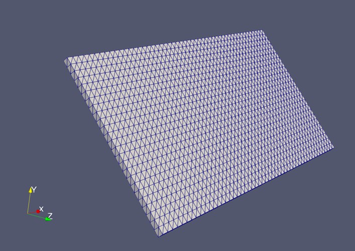
Figure 1. Wing/blade STL model with the mesh displayed.
Rotating Blade Simulation Using LBM–IBM
This project presents a numerical reconstruction of the rotating-wing experiment by Manar & Jones (2014) [1].
The simulation is implemented using the Lattice Boltzmann Method (LBM) coupled with the Immersed Boundary Method (IBM) to model rotating wings at low Reynolds numbers.
Although this setup originates from a classical experimental study, the goal here is not only to reproduce the original results but also to demonstrate how LBM–IBM can be applied to more general rotating-blade problems.
The simulation generates detailed flow fields, vortex structures, and pressure distributions that are difficult to capture experimentally, showing the potential of this method for applications such as:
In the original experiment, the wing (or blade) was attached to the rotation shaft using a very thin supporting rod.
In the numerical simulation, this auxiliary structure is unnecessary, since the wing can be rotated directly about its central axis. This is a practical advantage of the simulation: we are able to isolate the aerodynamic effects generated purely by the wing itself without the interference of any supporting components — an idealized condition that cannot be achieved in the physical experiment.
The solid wing used in this simulation is:
| Parameter | Value |
|---|---|
| chord $c$ | 7.62 cm |
| span $s$ | 15.24 cm |
| thickness $h$ | 0.254 cm |
Following the experimental setup, the wing is placed at a 45° angle of attack and rotates about a central shaft positioned \(r_t = 3.81\ \text{cm}\) away from the wing root.
Finally, the resulting geometry takes the form shown in Figure 1, and the corresponding MATLAB code is provided in the Appendix.
Figure 1. Wing/blade STL model with the mesh displayed.
In this simple resolution convergence check, a Reynolds number of \(Re = 500\) is used together with a constant angular velocity, whereas the original paper [1] employs a time-dependent angular velocity profile.
The Reynolds number is defined as follows:
where \(R_{75} = 0.75(r_t + s)\) and $\nu$ is the kinematic viscosity of the fluid.
Although $\Omega_{max}$ is introduced in the original paper as the maximum angular velocity in the transient profile, in the present resolution convergence study it is simply used as a constant angular velocity.
Simulations are conducted with 40 to 100 nodes along the spanwise direction, and the results are summarized below.
As shown in Figure 2, the simulation becomes mesh-independent as the resolution increases. Based on this convergence behavior, I finally choose \(N = 70\) as the resolution for all cases.
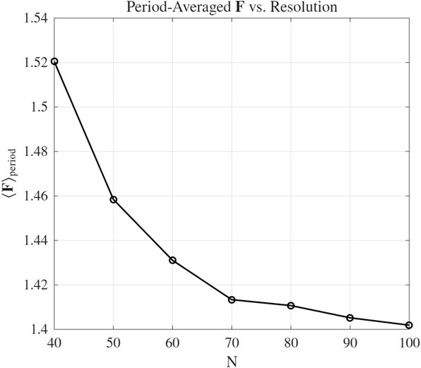
Figure 2. Average force during the 10th period as a function of resolution (force unit: Newton).
In the reference paper [1], the kinematics are divided into three phases:
During the acceleration and deceleration phases, the angular velocity varies linearly from zero to its maximum value, and then from the maximum value back to zero.
Because a sudden change in angular velocity would introduce infinite acceleration, a smoothing function is applied, as given in Equation 2. Here, $a$ is the smoothing parameter, which is set to \(a = 50\) following the original paper.
The parameters $t_1$, $t_2$, $t_3$, and $t_4$ denote the start and end times of the acceleration and deceleration phases, respectively.
The wing/blade completes two full revolutions, which leads to different values of $t_1$ through $t_4$ depending on the Reynolds number.
For convenience and reproducibility, these values are listed in Table 1, and the corresponding angular velocity profiles are shown in Figure 3.
| $Re$ | $\Omega_{max}$ | $t_1$ | $t_2$ | $t_3$ | $t_4$ |
|---|---|---|---|---|---|
| 120 | 0.671 | 0.300 | 0.363 | 19.032 | 19.096 |
| 500 | 2.795 | 0.300 | 0.315 | 4.796 | 4.811 |
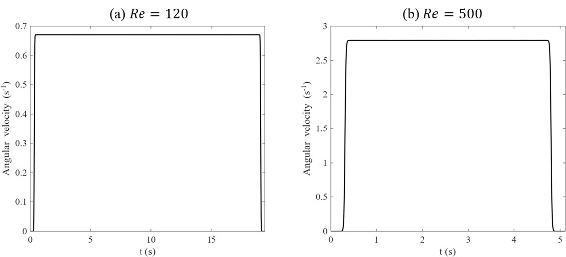
Figure 3. Angular velocity profile for Re= (a) 120 and (b) 500.
The animations below illustrate two types of simulations.
Constant case
Used for the resolution convergence check.
Transient case
Designed to reproduce the time-dependent motion described in the original paper.
Constant Case (Re = 120) Vorticity Field

Constant Case (Re = 500) Vorticity Field
Transient Case (Re = 120) Vorticity Field
Transient Case (Re = 500) Vorticity Field
It can be observed that in the Re = 120 case, the vortex remains primarily attached near the edge of the blade. In contrast, for Re = 500, the vortex structures extend throughout most of the computational domain. This suggests that mixing may be significantly enhanced at higher Reynolds numbers.
Further parametric studies could be conducted to identify the optimal geometry or rotational speed that maximizes mixing performance while minimizing energy consumption, allowing the mixing process to operate at an optimal efficiency.
The simulations were conducted using Palabos [2] together with our own rigid-body solver package.
The animations were generated using ParaView [3], while the geometry and prescribed transient motion were created using MATLAB [4] scripts.
The solid body solver package is not publicly available at this time.
Once potential conflicts of interest are resolved, we may consider releasing it as open-source in the future.
[1] Manar, F., & Jones, A. R. (2014). The effect of tip clearance on low Reynolds number rotating wings. AIAA Aerospace Sciences Meeting.
[2] J. Latt et al. Palabos: Parallel lattice Boltzmann solver. Computers & Mathematics with Applications, 81, 334–350 (2021).
[3] J. Ahrens, B. Geveci, and C. Law. ParaView: An End-User Tool for Large Data Visualization. The Visualization Handbook (2005).
[4] MATLAB, version R2024a. The MathWorks Inc., Natick, Massachusetts, United States.
clear; close all; clc; format long;

%% Global variables
Re = 500; % Desired Re number
c = 0.0762; % Wing chord
nu = 0.000060862; % Kinematic viscosity
% nu = 0.000008117; % Kinematic viscosity Re 1000
a = 50; % Paper specified a
tout = 0.3; % The time before acceleration and deacceleratio
tStep = 100000; % Resolution of the output angular velocity profile
outputDir = "./";

%% Calculation
% Necessary variables
s = c*2 % Wing span
root = c*0.5 % Root distance
R75 = 0.75*(s+root) % Radius
Omega_max = Re*nu/(R75*c) % Max angular velocity
tacc = 0.25*c/(2*pi*R75)*2/Omega_max % Acceleration time
tStable = (2*2*pi-2*0.25*c/(2*pi*R75))/Omega_max % Stable time

% Time and angular velocity calculation
t1 = tout;
t2 = t1+tacc;
t3 = t2+tStable;
t4 = t3+tacc;
t = t1-tout:(t4-t1)/tStep:t4+tout;
Omega = omega_profile(t, Omega_max, a, t1, t2, t3, t4);

% Plot
figure("Position", [100 100 600 500]);
set(groot, 'DefaultAxesFontName', 'Times New Roman');
set(groot, 'DefaultAxesFontSize', 14);
set(groot, 'DefaultTextFontName', 'Times New Roman');
set(groot, 'DefaultTextFontSize', 14);
set(groot, 'DefaultLineLineWidth', 1.5);
plot(t, Omega, "-k");
xlim([t1-tout t4+tout]);
xlabel("t (s)");
ylabel("Angular velocity (s^{-1})");

% Confirm it sweeps 2 revolutions
areaTotal = trapz(t, Omega); % Intergal
revolution = areaTotal/(2*pi)

% CSV Output
data = [t(:), Omega(:)];
csvFile = fullfile(outputDir, "profile.csv");
writematrix(data, csvFile);

fprintf("CSV file saved to: %s\n", csvFile);

%% Sub-functions
function Omega = omega_profile(t, Omega_max, a, t1, t2, t3, t4)
% OMEGA_PROFILE Smoothed angular velocity profile from Manar & Jones (2014)
%
%   Omega = omega_profile(t, Omega_max, a, t1, t2, t3, t4)
%
%   Implements the piecewise function:
%     For 0 <= t <= (t2+t3)/2:
%       Ω(t) = Ω_max/(2 a (t2-t1)) * log( cosh(a(t-t1))/cosh(a(t-t2)) ) + Ω_max/2
%     For (t2+t3)/2 <= t:
%       Ω(t) = -Ω_max/(2 a (t4-t3)) * log( cosh(a(t-t3))/cosh(a(t-t4)) ) + Ω_max/2
%
%   Inputs:
%     t         - time array (scalar or vector)
%     Omega_max - steady angular velocity (rad/s)
%     a         - smoothing parameter (paper uses a = 50)
%     t1        - start time of motion
%     t2        - end of acceleration
%     t3        - start of deceleration
%     t4        - end of deceleration
%
%   Output:
%     Omega     - angular velocity Ω(t) with same size as t

    % Pre-assignment
    Omega = zeros(size(t));

    % Switch time point
    t_switch = (t2 + t3)/2;

    % First section:Acc + Stable to mid point
    idx1 = (t >= 0) & (t <= t_switch);
    if any(idx1)
        tt = t(idx1);
        Omega(idx1) = Omega_max./(2*a*(t2 - t1)) .* ...
            log( cosh(a*(tt - t1)) ./ cosh(a*(tt - t2)) ) ...
            + Omega_max/2;
    end

    % Second section:Stable mid to the end
    idx2 = (t >= t_switch);
    if any(idx2)
        tt = t(idx2);
        Omega(idx2) = -Omega_max./(2*a*(t4 - t3)) .* ...
            log( cosh(a*(tt - t3)) ./ cosh(a*(tt - t4)) ) ...
            + Omega_max/2;
    end
end
%% generate_box_stl_xyz.m
% -------------------------------------------------------------------------
% Utility script to generate a rectangular box STL file.
%
% The box domain is defined as:
%       x : [0, L]
%       y : [0, W]
%       z : [0, H]
%
% nx, ny, nz represent the number of divisions in the x, y, z directions.
% The script generates a triangulated surface and writes a binary STL file.
% -------------------------------------------------------------------------

clear; clc; format long;

%% ===================== User-defined parameters ==========================
% Geometry dimensions
L  = 0.01*2.54*2.4;     % Length in x-direction
W  = 0.01*2.54*1.2;     % Width  in y-direction
H  = 0.01*2.54*0.07;    % Height in z-direction

% Base resolution
ny = 70;                % Resolution in y-direction
nx = ceil(ny/W*L);      % Resolution in x-direction (scaled with aspect ratio)
nz = ceil(ny/W*H);      % Resolution in z-direction

% Output STL filename
filename = 'wing.stl';

%% ====================== Resolution sanity check =========================
nx = max(1, round(nx));
ny = max(1, round(ny));
nz = max(1, round(nz));

fprintf('Generating box geometry: L = %.4g, W = %.4g, H = %.4g\n', L, W, H);
fprintf('Resolution: nx = %d, ny = %d, nz = %d\n', nx, ny, nz);
fprintf('Output STL file: %s\n', filename);

%% ===================== Triangle allocation ==============================
% Top/Bottom surfaces: 4 * nx * ny
% Front/Back surfaces: 4 * nx * nz
% Left/Right surfaces: 4 * ny * nz
numTris = 4 * (nx*ny + nx*nz + ny*nz);

% Each triangle stored as:
% [x1 y1 z1 x2 y2 z2 x3 y3 z3]
tris = zeros(numTris, 9);

idx = 1;

%% ======================== Grid generation ===============================
xs = linspace(0, L, nx+1);
ys = linspace(0, W, ny+1);
zs = linspace(0, H, nz+1);

%% ======================== Face 1 : Bottom (z = 0) =======================
% Normal direction: -z
z0 = 0;

for i = 1:nx
    for j = 1:ny

        x0 = xs(i);   x1 = xs(i+1);
        y0 = ys(j);   y1 = ys(j+1);

        p00 = [x0, y0, z0];
        p10 = [x1, y0, z0];
        p01 = [x0, y1, z0];
        p11 = [x1, y1, z0];

        tris(idx,:)   = [p00, p11, p10];
        tris(idx+1,:) = [p00, p01, p11];

        idx = idx + 2;

    end
end

%% ========================= Face 2 : Top (z = H) =========================
% Normal direction: +z
z0 = H;

for i = 1:nx
    for j = 1:ny

        x0 = xs(i);   x1 = xs(i+1);
        y0 = ys(j);   y1 = ys(j+1);

        p00 = [x0, y0, z0];
        p10 = [x1, y0, z0];
        p01 = [x0, y1, z0];
        p11 = [x1, y1, z0];

        tris(idx,:)   = [p00, p10, p11];
        tris(idx+1,:) = [p00, p11, p01];

        idx = idx + 2;

    end
end

%% ======================== Face 3 : Front (y = 0) ========================
% Normal direction: -y
y0 = 0;

for i = 1:nx
    for k = 1:nz

        x0 = xs(i);   x1 = xs(i+1);
        z0_ = zs(k);  z1_ = zs(k+1);

        p00 = [x0, y0, z0_];
        p10 = [x1, y0, z0_];
        p01 = [x0, y0, z1_];
        p11 = [x1, y0, z1_];

        tris(idx,:)   = [p00, p11, p10];
        tris(idx+1,:) = [p00, p01, p11];

        idx = idx + 2;

    end
end

%% ======================== Face 4 : Back (y = W) =========================
% Normal direction: +y
y0 = W;

for i = 1:nx
    for k = 1:nz

        x0 = xs(i);   x1 = xs(i+1);
        z0_ = zs(k);  z1_ = zs(k+1);

        p00 = [x0, y0, z0_];
        p10 = [x1, y0, z0_];
        p01 = [x0, y0, z1_];
        p11 = [x1, y0, z1_];

        tris(idx,:)   = [p00, p10, p11];
        tris(idx+1,:) = [p00, p11, p01];

        idx = idx + 2;

    end
end

%% ========================= Face 5 : Left (x = 0) ========================
% Normal direction: -x
x0 = 0;

for j = 1:ny
    for k = 1:nz

        y0 = ys(j);   y1 = ys(j+1);
        z0_ = zs(k);  z1_ = zs(k+1);

        p00 = [x0, y0, z0_];
        p10 = [x0, y1, z0_];
        p01 = [x0, y0, z1_];
        p11 = [x0, y1, z1_];

        tris(idx,:)   = [p00, p11, p10];
        tris(idx+1,:) = [p00, p01, p11];

        idx = idx + 2;

    end
end

%% ======================== Face 6 : Right (x = L) ========================
% Normal direction: +x
x0 = L;

for j = 1:ny
    for k = 1:nz

        y0 = ys(j);   y1 = ys(j+1);
        z0_ = zs(k);  z1_ = zs(k+1);

        p00 = [x0, y0, z0_];
        p10 = [x0, y1, z0_];
        p01 = [x0, y0, z1_];
        p11 = [x0, y1, z1_];

        tris(idx,:)   = [p00, p10, p11];
        tris(idx+1,:) = [p00, p11, p01];

        idx = idx + 2;

    end
end

%% ======================== Write binary STL ==============================
writeBinarySTL(filename, tris);

fprintf('STL file successfully generated: %s\n', filename);

%% ========================================================================
%% Function: Write Binary STL
%% ========================================================================
function writeBinarySTL(filename, tris)

numTris = size(tris,1);

fid = fopen(filename,'w','ieee-le');

if fid < 0
    error('Cannot open file: %s', filename);
end

% STL header (80 bytes)
header = zeros(1,80,'uint8');
fwrite(fid,header,'uint8');

% Number of triangles
fwrite(fid,uint32(numTris),'uint32');

for i = 1:numTris

    v1 = tris(i,1:3);
    v2 = tris(i,4:6);
    v3 = tris(i,7:9);

    % Compute surface normal
    n = cross(v2-v1, v3-v1);

    nNorm = norm(n);

    if nNorm > 0
        n = n / nNorm;
    else
        n = [0 0 0];
    end

    fwrite(fid,single(n),'float32');
    fwrite(fid,single(v1),'float32');
    fwrite(fid,single(v2),'float32');
    fwrite(fid,single(v3),'float32');

    % Attribute byte count
    fwrite(fid,uint16(0),'uint16');

end

fclose(fid);

end